Example: Connected springs
This example is from the CALFEM manual (exs1.py).
Purpose:
Show the basic steps in a finite element calculation.
Description:
The general procedure in linear finite element calculations is carried out for a simple structure. The steps are:
define the model
generate element matrices
assemble element matrices into the global system of equations
solve the global system of equations
evaluate element forces
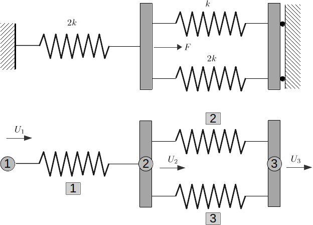
Consider the system of three linear elastic springs, and the corresponding finite element model. The system of springs is fixed in its ends and loaded by a single load F. To make it convenience, we follow notation in “Fundamentals of Finite Element Analysis” by David Hutton, where square is symbol for nodes, circle is for element, and U is for (global) nodal displacement. Capital letter shows global variables while small letter follows local variables.
We begin our FEM computation by importing required modules
# ----- import necesarry mooules
The computation is initialized by defining the topology matrix Edof, containing element numbers and global element degrees of freedom. All input to CALFEM is NumPy arrays. Topology is defined by index 1, i.e., the first row represents the first element bounded by node 1 and node 2. Hence we write
import calfem.core as cfc
import calfem.utils as cfu

# ----- Topology matrix Edof
the initial global stiffness matrix K (3x3) and load force f containing zeros,
    [2, 3],      # element 2 between node 2 and 3
    [2, 3]       # element 3 between node 2 and 3
Element stiffness matrices are generated by the function spring1e. The element property ep for the springs contains the spring stiffnesses k and 2k respectively, where k = 1500.
# ----- Stiffness matrix K and load vector f

K = np.zeros((3, 3))
f = np.zeros((3, 1))

# ----- Element stiffness matrices

k = 1500.
ep1 = k
ep2 = 2.*k
Ke1 = cfc.spring1e(ep1)
Ke2 = cfc.spring1e(ep2)
The output is printed as follows:
Stiffness matrix K:
[[ 3000. -3000.     0.]
 [-3000.  7500. -4500.]
 [    0. -4500.  4500.]]
and the load/force vector f (3x1) with the load F = 100 in position 2 (Note that Python indexes from 0, hence f[1] corresponds to edof 2).
cfc.assem(edof[0, :], K, Ke2)
The element stiffness matrices are assembled into the global stiffness matrix K according to the topology. bc is an array of prescribed degrees of freedom. Values to be specified are specified in a separate array. If all values are 0, they don’t have to be specified. The global system of equations is solved considering the boundary conditions given in bc.
cfu.disp_h2("Stiffness matrix K:")
cfu.disp_array(K)

# f[1] corresponds to edof 2

f[1] = 100.0
output:
Displacements a:
[[0.        ]
 [0.01333333]
 [0.        ]]
Reaction forces Q:
[[-40.]
 [  0.]
 [-60.]]
Element forces are evaluated from the element displacements. These are obtained from the global displacements a using the function extract.
bc = np.array([1, 3])
a, r = cfc.solveq(K, f, bc)
The spring element forces at each element are evaluated using the function spring1s.
# ----- Caculate element forces

ed1 = cfc.extract_ed(edof[0, :], a)
Output:
Element forces N:
N1 = 40.0
N2 = -20.0
N3 = -40.0