Example: More bars

This example is from Calfem manual (exs4.py).

Purpose:

Analysis of a plane truss.

Description:

Consider a plane truss, loaded by a single force P = 0.5 MN at 30 \(^\circ\) from normal.

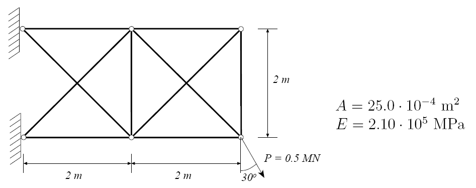
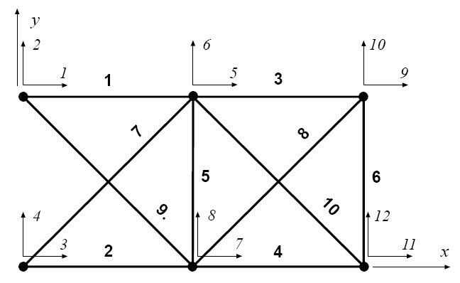
The corresponding finite element model consists of ten elements and twelve degrees of freedom.

First, import necessart modules.

import numpy as np
import calfem.core as cfc

The topology is defined by the matrix

Edof = np.array([
    [1, 2, 5, 6],
    [3, 4, 7, 8],
    [5, 6, 9, 10],
    [7, 8, 11, 12],
    [7, 8, 5, 6],
    [11, 12, 9, 10],
    [3, 4, 5, 6],
    [7, 8, 9, 10],
    [1, 2, 7, 8],
    [5, 6, 11, 12]
])

A global stiffness matrix K and a load vector f are defined. The load P is divided into x and y components and inserted in the load vector f.

K = np.zeros([12,12])
f = np.zeros([12,1])

The element matrices Ke are computed by the function bar2e. These matrices are then assembled in the global stiffness matrix using the function assem.

A = 25.0e-4
E = 2.1e11
ep = [E,A]

Element coordinates are defined as follows.

ex = np.array([
    [0., 2.],
    [0., 2.],
    [2., 4.],
    [2., 4.],
    [2., 2.],
    [4., 4.],
    [0., 2.],
    [2., 4.],
    [0., 2.],
    [2., 4.]
])

ey = np.array([
    [2., 2.],
    [0., 0.],
    [2., 2.],
    [0., 0.],
    [0., 2.],
    [0., 2.],
    [0., 2.],
    [0., 2.],
    [2., 0.],
    [2., 0.]
])

All the element matrices are computed and assembled in the loop.

for elx, ely, eltopo in zip(ex, ey, Edof):
    Ke = cfc.bar2e(elx, ely, ep)
    cfc.assem(eltopo, K, Ke)

The displacements in a and the support forces in r are computed by solving the system of equations considering the boundary conditions in bc.

bc = np.array([1,2,3,4])

f[10]=0.5e6*np.sin(np.pi/6)
f[11]=-0.5e6*np.cos(np.pi/6)

a, r = cfc.solveq(K,f,bc)

print("Displacement: ")
print(a)

Displacement:
[[ 0.        ]
 [ 0.        ]
 [ 0.        ]
 [ 0.        ]
 [ 0.00238453]
 [-0.0044633 ]
 [-0.00161181]
 [-0.00419874]
 [ 0.00303458]
 [-0.01068377]
 [-0.00165894]
 [-0.01133382]]

print("Support force: ")
print(r)

Support force:
[[-8.66025404e+05]
 [ 2.40086918e+05]
 [ 6.16025404e+05]
 [ 1.92925784e+05]
 [ 4.65661287e-10]
 [-2.91038305e-11]
 [ 1.16415322e-10]
 [ 1.16415322e-10]
 [-4.65661287e-10]
 [ 3.49245965e-10]
 [-2.03726813e-10]
 [ 4.65661287e-10]]

The displacement at the point of loading is \(−1.7 · 10^{−3} m\) in the x-direction and \(−11.3 · 10^{−3} ~m\) in the y-direction. At the upper support the horizontal force is \(−0.866~MN\) and the vertical \(0.240 ~MN\). At the lower support the forces are \(0.616~MN\) and \(0.193~MN\), respectively. Normal forces are evaluated from element displacements. These are obtained from the global displacements a using the function extract. The normal forces are evaluated using the function bar2s.

ed = cfc.extractEldisp(Edof,a)

N = np.zeros([Edof.shape[0]])

print("Element forces:")

i = 0
for elx, ely, eld in zip(ex, ey, ed):
    N[i] = cfc.bar2s(elx, ely, ep, eld)
    print("N%d = %g" % (i+1,N[i]))
    i+=1

Element forces:
N1 = 625938
N2 = -423100
N3 = 170640
N4 = -12372.8
N5 = -69447
N6 = 170640
N7 = -272838
N8 = -241321
N9 = 339534
N10 = 371051

The largest normal force N = 0.626 MN is obtained in element 1 and is equivalent to a normal stress σ = 250 MPa.

To reduce the quantity of input data, the element coordinates matrices Ex and Ey can alternatively be created from a global coordinate matrix Coord and a global topology matrix Dof using the function coordxtr, i.e.

Coord = np.array([
[0, 2],
[0, 0],
[2, 2],
[2, 0],
[4, 2],
[4, 0]
])

Dof = np.array([
[1, 2],
[3, 4],
[5, 6],
[7, 8],
[9, 10],
[11, 12]
])

ex, ey = cfc.coordxtr(Edof, Coord, Dof)

print(ex)

array([[0., 2.],
       [0., 2.],
       [2., 4.],
       [2., 4.],
       [2., 2.],
       [4., 4.],
       [0., 2.],
       [2., 4.],
       [0., 2.],
       [2., 4.]])

print(ey)

array([[2., 2.],
       [0., 0.],
       [2., 2.],
       [0., 0.],
       [0., 2.],
       [0., 2.],
       [0., 2.],
       [0., 2.],
       [2., 0.],
       [2., 0.]])

As can be seen above, ex and ey is same as previous.